
You’ve probably stared at a loss curve that looks like a rollercoaster during your last Large Language Model (LLM) training run. One minute it’s dropping beautifully; the next, it spikes or flatlines entirely. If you’re working with deep transformers, the culprit is rarely your data-it’s usually how you’re handling activation values as they flow through dozens of layers. This is where Layer Normalization (LayerNorm) and residual paths step in. They aren’t just academic footnotes; they are the engineering glue keeping billion-parameter models from exploding into NaNs.
If you want to train stable models without burning weeks on hyperparameter tuning, you need to understand exactly how normalization interacts with residual connections. We’ll break down why standard LayerNorm works, why the industry shifted to Pre-LayerNorm configurations, and whether newer tricks like RMSNorm are actually worth your time. By the end, you’ll know which setup fits your specific model size and hardware constraints.
The Core Problem: Why Deep Networks Explode
Imagine passing information through 60 layers of neural networks. In each layer, weights multiply inputs, and biases add noise. Without control, these operations compound. Small changes amplify exponentially. This leads to two nightmares for ML engineers: vanishing gradients (where learning stops because updates become infinitesimally small) and exploding activations (where values become so large they overflow memory or destabilize math).
Layer Normalization solves this by forcing each sample’s feature vector to have a mean of zero and a variance of one before proceeding. Unlike Batch Normalization, which relies on batch statistics and fails with variable-length sequences common in NLP, LayerNorm operates independently on each token. It normalizes across the feature dimension, not the batch dimension. This independence makes it ideal for transformer architectures where sequence lengths vary wildly between samples.
The formula looks intimidating but is straightforward: y = γ × (x - μ) / √(σ² + ε) + β. Here, μ and σ² are calculated per-sample across features. The learnable parameters γ (scale) and β (bias) allow the network to undo the normalization if it hinders performance. This mechanism stabilizes the internal distribution of activations, allowing for higher learning rates and faster convergence.
Pre-LN vs. Post-LN: The Great Architectural Shift
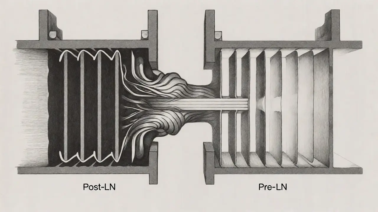
Originally, the Transformer paper used Post-LayerNorm, placing normalization after the residual connection. For shallow models, this worked fine. But as we scaled to GPT-2 and beyond, Post-LN became unstable. Research shows that in Post-LN architectures, variance grows massively in deeper layers-up to 470% growth by layer 60 in some experiments. This phenomenon, known as "massive activations," disrupts gradient flow.
Enter Pre-LayerNorm. By moving the normalization step before the attention and feed-forward blocks, the residual path remains unnormalized. This creates a clean identity path for gradients to flow back through the network. The impact is significant. Studies indicate Pre-LN provides 7% to 64% faster training convergence compared to Post-LN for deep networks. Major players like OpenAI (GPT-2), Google (T5), and DeepMind (PaLM) all adopted Pre-LN strategies for their flagship models.
| Feature | Post-LayerNorm | Pre-LayerNorm | RMSNorm |
|---|---|---|---|
| Normalization Location | After residual addition | Before sub-layers | Before sub-layers (No mean subtraction) |
| Training Stability | Low for >32 layers | High for >100 layers | High, comparable to Pre-LN |
| Computational Cost | Moderate | Moderate | Low (12.7% faster on A100) |
| Gradient Flow | Prone to vanishing/exploding | Stable via identity path | Stable, rescaling invariant |
| Industry Adoption | Legacy models | GPT-2, T5, PaLM | Llama, Mistral, Modern LLMs |
RMSNorm: The Efficiency Upgrade
If LayerNorm calculates both mean and variance, RMSNorm skips the mean subtraction entirely. Introduced by Zhang and Sennrich in 2019, it normalizes only by the root mean square value: y = γ × x / √(RMS(x)² + ε). Why does this matter? Calculating the mean requires an extra pass over the data, consuming memory bandwidth. On modern GPUs like the NVIDIA A100, eliminating this step yields approximately 12.7% faster computation for the normalization layer itself.
Beyond speed, RMSNorm offers "rescaling invariance." If you scale the input, the output scales proportionally. This property helps maintain stability during distributed training, where different workers might process slightly different data distributions. Google’s T5 implementation reported 7-9% faster overall training times using RMSNorm. However, there’s a catch. Because RMSNorm doesn’t center the data around zero, it lacks the symmetry of LayerNorm. Some practitioners report needing to lower learning rates by 5-10% when switching to RMSNorm to avoid instability.
Community feedback highlights this trade-off. On forums like Reddit’s r/MachineLearning, users report 8-12% faster training on 7B-parameter models with RMSNorm, but warn of convergence issues if learning rates exceed 2e-4. If you’re fine-tuning smaller models (<1B parameters), the difference between LayerNorm and RMSNorm is often negligible. But for massive pre-training runs, those percentage points translate to thousands of dollars in cloud compute savings.
Residual Paths: The Highway for Gradients
Normalization alone isn’t enough. You need robust residual connections. These skip connections add the input directly to the output of a sub-layer, creating a shortcut for gradients. In Pre-LN setups, the residual path is pure identity until the final layer. This ensures that even if the attention block learns nothing useful, the signal still passes through unchanged.
However, naive residual connections can lead to variance accumulation. Each layer adds its own transformation to the sum. Over 80 layers, this sum can drift significantly. Recent research proposes Peri-LayerNorm (Peri-LN), which places normalization both before and after the residual connection. This dual-placement strategy reduces gradient spikes by 52% compared to standard Pre-LN. While Peri-LN shows promise in experimental settings (like DeepMind’s tests on 3.2B parameter models), it hasn’t yet seen widespread adoption in production open-source models like Llama-3 or Mistral.
For most developers today, sticking to standard Pre-LN with RMSNorm is the safest bet. It balances proven stability with computational efficiency. If you’re building a custom architecture exceeding 100 layers, consider experimenting with Peri-LN or careful scaling factors on the residual paths to prevent variance explosion.
Implementation Pitfalls and Best Practices
Even with the right theory, implementation bugs creep in. A common mistake identified in Hugging Face GitHub issues is inconsistent normalization placement between training and inference. Ensure your code applies the same logic in both phases. Another frequent issue involves the epsilon value (ε) in the denominator. Standard implementations use 1e-5, but in mixed-precision training (FP16/BF16), this can cause underflow errors. Increasing epsilon to 1e-6 or 1e-8 depending on precision levels can resolve NaN losses.
- Check Epsilon Values: Adjust
εbased on your floating-point precision (FP16 vs FP32). - Monitor Activation Variance: Log the variance of outputs at every 10th layer. If it grows exponentially, your normalization is failing.
- Warm Up Gamma: Start with small initial values for the scale parameter
γ(e.g., 0.1) and gradually increase it to 1.0 over the first few thousand steps. This "warmup" technique reduces early training instability by up to 37%. - Consistency Matters: Do not change normalization types mid-training. Switching from LayerNorm to RMSNorm requires re-initializing weights or extensive fine-tuning.
Hardware constraints also play a role. If you’re training on memory-bandwidth-limited devices (like older consumer GPUs), RMSNorm’s reduced memory access patterns provide a tangible benefit. Conversely, if you have abundant compute but limited VRAM, the slight accuracy dip from RMSNorm might be acceptable to fit larger batch sizes.
The Future: Will Normalization Disappear?
A provocative 2023 study titled "Transformers Don’t Need LayerNorm at Inference Time" suggests that once a model is trained, you can remove normalization layers entirely with minimal performance loss (only 0.03 cross-entropy increase on GPT-2 XL). This implies normalization is primarily a training aid, not a functional requirement.
Emerging techniques like Dynamic Thresholding (DyT) aim to eliminate explicit normalization layers altogether. DyT achieves comparable accuracy while improving inference speed by 14.2%. Industry leaders are watching closely. Meta’s team reportedly explored normalization-free directions for Llama-3, though they ultimately retained standard approaches for reliability. The consensus among researchers is that while explicit normalization may fade, some form of implicit stabilization will remain essential for models exceeding 500 billion parameters.
For now, don’t try to reinvent the wheel. Use Pre-LN with RMSNorm. It’s the sweet spot of stability, speed, and community support. Keep an eye on Peri-LN and DyT for future architectures, but master the current standards first.
Why is Pre-LayerNorm preferred over Post-LayerNorm?
Pre-LayerNorm provides more stable gradient flow, especially in deep networks (>32 layers). It prevents "massive activations" by keeping the residual path unnormalized, allowing for faster convergence and higher learning rates compared to Post-LayerNorm.
What is the main advantage of RMSNorm over LayerNorm?
RMSNorm eliminates the mean subtraction step, reducing computational cost and memory bandwidth usage. This results in approximately 12.7% faster computation on modern GPUs like the NVIDIA A100, making it ideal for large-scale training.
Can I remove LayerNorm during inference?
Yes, recent studies show that removing LayerNorm during inference incurs minimal performance loss (e.g., 0.03 cross-entropy increase). Normalization primarily aids training stability rather than being critical for the final model's functionality.
How do I handle NaN losses with RMSNorm?
NaN losses often stem from division by near-zero values. Increase the epsilon value (ε) in the RMSNorm formula, typically to 1e-6 or 1e-8 depending on precision. Also, ensure your learning rate is adjusted downward by 5-10% when switching to RMSNorm.
Is Peri-LayerNorm ready for production use?
Peri-LayerNorm shows promising results in research, offering better stability than Pre-LN. However, it is not yet widely adopted in major open-source models like Llama or Mistral. It is best suited for experimental architectures or very deep custom models.