You’ve built your large language model. It’s smart, it’s responsive, and it answers questions with impressive nuance. But then you try to serve it to real users, and everything falls apart. The GPU memory fills up instantly. Latency spikes when multiple people ask questions at once. Your costs skyrocket because the server is idle half the time but burns power the other half. This isn’t a failure of your model architecture; it’s a failure of your inference infrastructure.
The gap between training an Large Language Model (a deep learning model trained on massive datasets to understand and generate human language) and serving it efficiently is where most projects die. To bridge this gap, you need two specific engineering tricks that have become non-negotiable in modern AI deployment: KV caching and Continuous Batching (an optimization technique that dynamically manages request queues to maximize GPU utilization during LLM inference). These aren't just nice-to-have optimizations anymore. As of mid-2026, they are the baseline for any production-grade LLM service. If you aren't using them, you're leaving money on the table and frustrating your users.
Why Standard Transformer Inference Fails at Scale
To understand why these tricks matter, you first need to see what happens inside a standard transformer during generation. Transformers work autoregressively. They predict one token at a time. When generating the second word, the model looks at the first. When generating the third, it looks at the first two. And so on.
In a naive implementation, every time the model generates a new token, it recomputes the attention mechanism for all previous tokens. If you’re generating a sentence with 100 words, by the time you reach the last word, the model has processed the entire history 99 times. This redundancy creates a computational complexity of O(n²) per step. For short prompts, this is manageable. But for long conversations or document analysis, it becomes prohibitively slow and expensive.
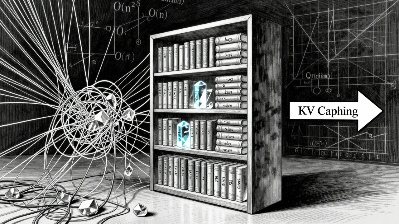
Imagine reading a book. Every time you start a new paragraph, instead of remembering the plot from the previous chapter, you re-read the entire book from page one. That’s naive transformer inference. It’s exhausting, inefficient, and unsustainable. KV caching fixes this by giving the model a memory bank.
How KV Caching Solves the Redundancy Problem
KV Caching (a technique that stores previously computed key and value vectors in memory to avoid redundant calculations during autoregressive generation) changes the game by storing the "keys" and "values" computed for each token after the first pass. When the model needs to attend to previous context for the next token, it doesn’t recompute those keys and values. It pulls them from the cache.
This shifts the computational complexity from O(n²) to O(n) per token. According to benchmarks from NVIDIA in early 2025, this reduction allows for practical generation of long sequences that were previously impossible on consumer hardware. For a model like LLaMA-3 8B processing a sequence of 2,000 tokens with a batch size of 16, the KV cache can contain over 8 billion elements-more data than the model’s own parameters.
| Sequence Length | Batch Size | Approximate KV Cache Memory | Model Weights Memory |
|---|---|---|---|
| 2,048 tokens | 1 | ~1.2 GB | ~16 GB |
| 8,192 tokens | 1 | ~4.8 GB | ~16 GB |
| 32,768 tokens | 1 | ~19.2 GB | ~16 GB |
| 32,768 tokens | 16 | ~307 GB | ~16 GB |
As you can see, the cache grows linearly with sequence length and batch size. At 32k tokens, the cache alone exceeds the model weights. This is the primary bottleneck in LLM serving. The memory footprint formula is roughly: `2 × hidden_size × num_layers × num_heads × sequence_length × precision_bytes`. For a typical 7B parameter model at FP16 precision, processing 32k tokens requires about 13.4 GB of VRAM just for the cache.
The Memory Crisis and Compression Solutions
If KV caching is so efficient computationally, why is it such a headache? Because memory is finite. GPUs have limited High Bandwidth Memory (HBM). When the KV cache fills up, you hit a wall. NVIDIA reported in Q2 2025 that 68% of attempted LLM deployments failed due to KV cache memory constraints. You can’t just add more RAM; the bandwidth between CPU and GPU is too slow. Offloading cache to host memory adds 18-22ms of latency per transfer, which kills the user experience.
To solve this, the industry has moved toward aggressive compression techniques. Here are the three main approaches dominating the landscape in 2026:
- NVFP4 Quantization: Developed by NVIDIA, this reduces the precision of cached values from FP16 (16-bit) to FP4 (4-bit). It cuts memory usage by 50% with less than 1% accuracy loss across most benchmarks. However, it requires Blackwell architecture GPUs (like the RTX 6000 Ada) to run efficiently. If you’re on older hardware, this option is off the table.
- SpeCache: An open-source approach that uses speculative caching. Instead of storing every key-value pair, it predicts which pairs are most important for future attention and prefetches only those. Research by Wang et al. (March 2025) showed this achieves 2.3× compression with a negligible 0.8% increase in perplexity. It’s particularly effective for reducing CPU-GPU transfer overhead.
- KVzip: A method that enables 3-4× reduction in cache size with negligible performance loss up to 170K context lengths. It’s ideal for applications requiring extremely long contexts, such as legal document analysis or codebase summarization.
While these methods save space, they introduce trade-offs. NVFP4 shows a 0.9% accuracy drop on MMLU benchmarks. SpeCache can suffer from reconstruction latency if predictions are wrong. You must choose based on your application’s tolerance for error versus its need for speed and cost efficiency.
Continuous Batching: Keeping the GPU Busy
Even with perfect KV caching, you face another problem: variance. LLM requests are not uniform. Some users ask short questions; others paste entire essays. Some responses are generated quickly; others take minutes. Traditional static batching groups requests together and waits for the slowest one to finish before starting the next batch. This leaves the GPU idle while waiting for fast requests to catch up with slow ones.
Continuous Batching (a dynamic scheduling algorithm that inserts new requests into the batch as soon as previous requests complete, rather than waiting for the entire batch to finish) solves this by treating the batch as a fluid queue. When one request finishes generating its response, the system immediately slots in a new pending request into that slot. The GPU never sits idle.
Frameworks like vLLM (an open-source library for high-throughput and memory-efficient LLM inference and serving) have made continuous batching accessible. In version 0.5.1 (released late 2025), vLLM demonstrated 3.8× higher throughput compared to non-batched serving for concurrent requests. However, this comes with a caveat: individual request latency variance increases by 22-27%. Some users might experience slightly longer wait times if the system is heavily loaded, but the overall system capacity improves dramatically.
Implementing the Stack: Practical Steps
So how do you actually put this into practice? You don’t need to build these systems from scratch. The ecosystem has matured significantly. Here is a realistic path to implementation for a developer in 2026.
- Choose Your Serving Engine: Don’t write your own scheduler. Use established frameworks. vLLM is the market leader for open-source implementations, holding 31% of the enterprise stack share. Text Generation Inference (TGI) (an open-source library developed by Hugging Face for deploying and serving Large Language Models) is a strong alternative, especially if you’re already deep in the Hugging Face ecosystem. For proprietary solutions, NVIDIA’s TensorRT-LLM offers tight integration with their hardware.
- Configure Cache Size: Allocate 50-70% of your available VRAM to the KV cache. If you allocate too little, you’ll evict pages frequently, causing latency spikes. Too much, and you can’t fit enough batches to utilize the GPU. Start with 60% and monitor eviction rates.
- Select Precision Strategy: If you have Blackwell GPUs, enable NVFP4. It’s the easiest win for doubling your context budget. If you’re on Ampere or older, stick to FP16 but implement SpeCache or KVzip via plugin support in vLLM. Avoid FP8 unless you’ve tested it thoroughly on your specific dataset, as quantization artifacts can degrade creative writing tasks.
- Enable Continuous Batching: In vLLM, this is often enabled by default. Ensure your maximum batch size is set high enough to absorb traffic bursts. Monitor the “preemption rate” metric. If preemptions are frequent, your batch size is too small relative to your request volume.
- Monitor Tail Latency: Average latency lies. Focus on p95 and p99 latency. Continuous batching can cause tail latency spikes. If your p99 latency exceeds acceptable thresholds, consider implementing request prioritization or separate queues for urgent vs. background tasks.
The Trade-Offs You Can’t Ignore
No solution is free. Implementing these tricks introduces complexity. Microsoft Research noted in September 2025 that current KV compression techniques can introduce non-negligible quality degradation for creative tasks, with perplexity increases of 3-5% on story generation benchmarks. If your application relies on nuanced, creative output, aggressive compression might make your model sound robotic or inconsistent.
Additionally, managing these systems requires expertise. Lambda Labs’ training data from Q4 2025 suggests developers typically need 2-3 weeks to master advanced KV cache management. You’ll need to understand CUDA programming basics and transformer internals to troubleshoot issues like non-contiguous memory transfers, which can add 15-18% overhead in PyTorch if not handled correctly.
There’s also a regulatory angle emerging. The EU’s AI Office draft guidelines from November 2025 require transparency about accuracy impacts from KV cache compression in high-risk applications. If you’re deploying medical or legal advice models, you may need to disable certain compression features to comply with upcoming regulations.
Future Outlook: What’s Next?
The trajectory is clear. Gartner predicts that KV cache optimization will be standard in all commercial LLM serving stacks by 2026, reducing infrastructure costs by 35-40%. We’re already seeing this happen. Enterprise users at Scale AI reported achieving 4.1× higher throughput after implementing NVFP4 quantization. Anthropic engineers noted a $2.3M monthly reduction in infrastructure costs through cache compression.
Looking ahead, Meta has announced dynamic cache resizing for Llama 4 in Q2 2026, which will allow the cache to expand and contract automatically based on load. Google DeepMind is exploring cache-aware transformer designs that could reduce memory requirements by an additional 3-5×. The goal is to make KV caching invisible-to handle it seamlessly without manual tuning.
For now, however, it remains a manual art. You must balance memory, speed, and accuracy. But the tools are here. The knowledge is available. The question is no longer whether you can afford to optimize your LLM serving, but whether you can afford not to.
What is the difference between static batching and continuous batching?
Static batching processes a fixed group of requests together and waits for the slowest request to finish before starting the next batch. This leads to GPU idle time. Continuous batching dynamically inserts new requests into the batch as soon as previous requests complete, keeping the GPU fully utilized and increasing overall throughput, though it may increase variance in individual request latency.
Does KV caching work with all transformer models?
Yes, KV caching is compatible with any autoregressive transformer model, including LLaMA, Mistral, Falcon, and GPT architectures. It is a fundamental optimization for the attention mechanism used in these models. However, the memory savings depend on the model's hidden size, number of layers, and head count.
Can I use NVFP4 quantization on older GPUs?
No, NVFP4 requires NVIDIA Blackwell architecture GPUs (such as the RTX 6000 Ada or newer) to leverage hardware-accelerated mixed-precision operations. On older architectures like Ampere or Turing, you would need to rely on software-based quantization (like FP8) or compression techniques like SpeCache, which may incur higher latency overhead.
How much memory does KV cache consume for a 7B parameter model?
For a 7B parameter model at FP16 precision, processing a sequence of 32,768 tokens consumes approximately 13.4 GB of VRAM for the KV cache alone. This does not include the memory required for the model weights themselves, which typically require around 14-16 GB. Therefore, serving such a model with long contexts requires a GPU with at least 24-32 GB of VRAM.
Is vLLM the best framework for continuous batching?
vLLM is currently one of the most popular and performant open-source frameworks for continuous batching, holding significant market share. However, alternatives like Hugging Face's Text Generation Inference (TGI) and NVIDIA's TensorRT-LLM are also highly capable. The best choice depends on your existing infrastructure, hardware compatibility, and specific feature requirements.


